🔎 Capital Structure big picture

This is the first lecture in a two lecture sequence to how much debt a company should have. Our goal is to maximize the value of the firm to maximize the wealth of the current owners. Therefore, we look at the value of the firm with various amounts of leverage. We choose the amount of debt that maximizes the value of the firm, V^L.

This week is just laying a foundation. Next week we’ll see that the optimal amount of debt involves a tradeoff between the tax advantages of debt and the downsides of debt. Other factors are also involved.

These tradeoffs are summarized in the “tradeoff theory” of optimal leverage. It is summarized in the following diagram. (The slide it’s on will likely be presented next week, so you are not responsible for it at this point. The goal is just to help you get a sense of how this fits in to Bruce’s larger plan.)

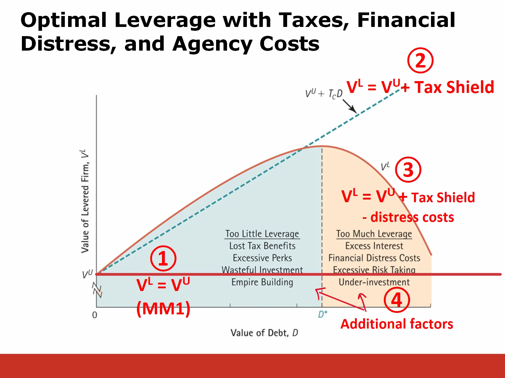
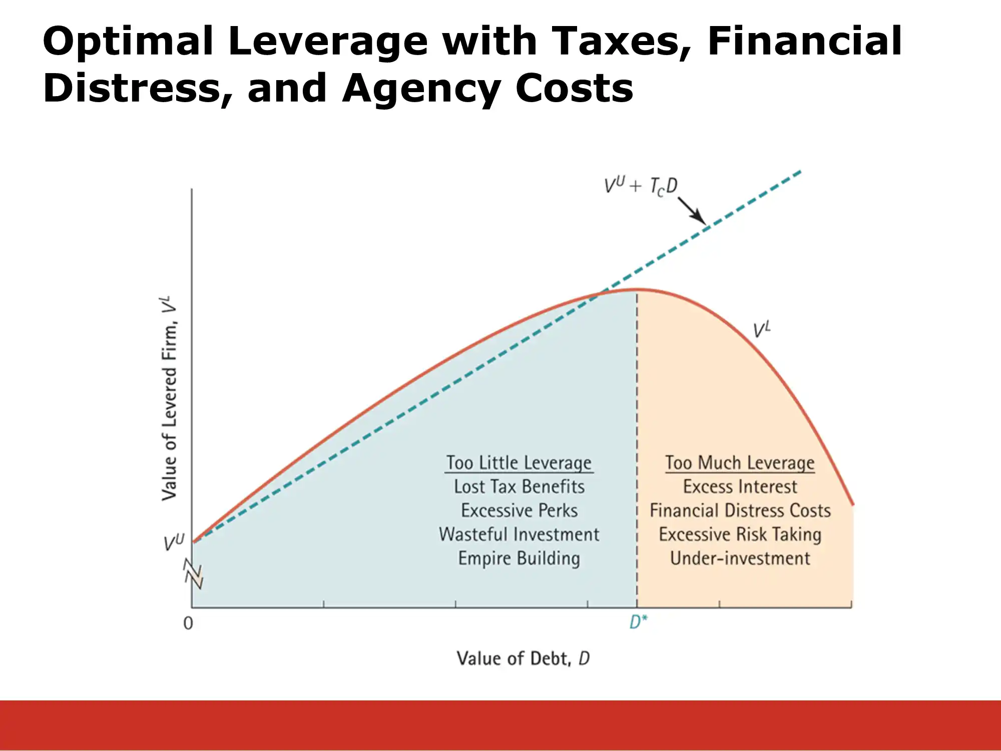
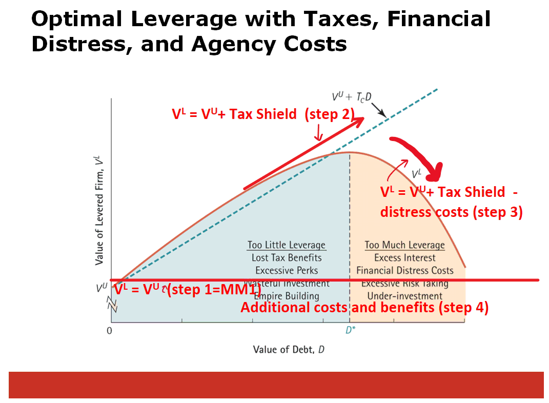
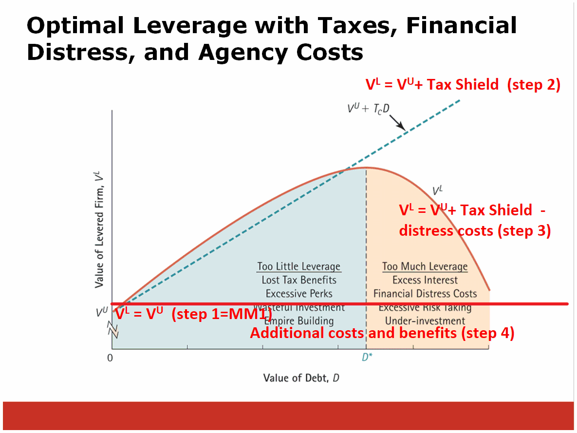
The diagram is a plot of the value of the levered firm (V^L) vs the total amount of debt the firm has (D). You can see that V^L, the red line, has a peak at an optimal level of debt, D*.

To identify D*, the full analysis has four steps. For each step, I’ve show where they are indicated in the diagram below. So far, we only have done the first two steps:

Step 1: First, we see that under idealized circumstances, the value of a firm doesn’t depend on D. Specifically, MM1 tells us that for any level of D, V^L=V^U. This is indicated by the horizontal red line near the bottom of the diagram. We use MM1 as our baseline (both literally and figuratively)

Step 2: Next, we see that debt provides a tax shield that increases the value of the firm. The more debt, the better. This is indicated by the dotted bluish line that slopes up with more debt.

Step 3: Unfortunately, debt can be risky. This leads to distress costs, which cause the red line to slope downward.

Step 4: Finally, we analyze additional factors in step 4.

Bruce will explain the third and fourth steps in the following lecture, so I have heavily abbreviated them here.

(I’ll explain the following diagram in section, but you can skip it if just reading.)

MM1

At this point, all we have is the first M&M theory. The first M&M theory says that the Value of the levered firm, $V^L$ doesn’t depend on the amount of debt at all. (under certain assumptions) Specifically, MM1 says that no matter how much debt the firm has, $V_L = V_U$ - ie that the value of the levered firm equals the value of the unlevered firm. (The value of the Levered firm is just defined as the value of the debt plus the value of the equity, building off of the “Corporate Finance Perspective” that we discussed in an earlier section. ie $V_L = E + D = V_U$ )

MM Proposition 1: In a perfect capital market, the total value of a firm is equal to the market value of the free cash flows generated by its assets and is not affected by its choice of capital structure.

V^L = E + D = V^U

Put very simply, MM1 says, “Lever up all you want or not at all… it won’t change the value of the firm!”

The problem is the assumptions. We’re going to relax the assumptions later. By starting with MM1 and relaxing it’s assumptions, we will be able to figure out D* - the optimal amount of debt for the firm to have (warning: we won’t have a precise number - this is just a framework for understanding the factors that determine D*)

MM2

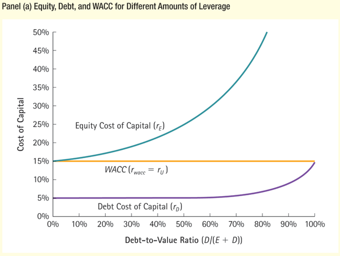
MM2 is the flip side of MM1. Rather than looking at the total value of the firm, it talks about how much the owners of the firm must pay to raise additional capital (ie the firm’s cost of capital). MM Proposition II: Cost of levered equity equals the cost of unlevered equity plus a premium proportional to the debt-equity ratio

r_E = r_U + \frac{D}{E}(r_u - r_D)

Notation reference:

In words	notation	also known as
return on levered equity	r_E	cost of levered equity
return on unlevered equity	r_U	cost of unlevered equity
return on debt	r_D	interest rate or cost of debt
market value of debt	D
market value of equity	E	D/E = debt-equity ratio

Just like MM1, it says, that under these assumptions the amount of debt doesn’t matter. MM2 says that the WACC will always be the same. This is illustrated in the following chart. As the Debt-to-Value ratio increases, note that the WACC doesn’t change at all! The WACC is completely constant.

Tax Shields

Because interest payments can decrease pretax income, they provide a tax shelter. This tax shelter can increase the value of the levered firm from $V^U$ to $V^U + T_CD$ , where $T_C$ is the corporate tax rate and D is the total market value of debt. This is illustrated by the dashed bluish line in the diagram below. Its upward slope indicates that the tax shield adds more and more value as the amount of debt increases:

Steps 1-3 of the Tradeoff Theory

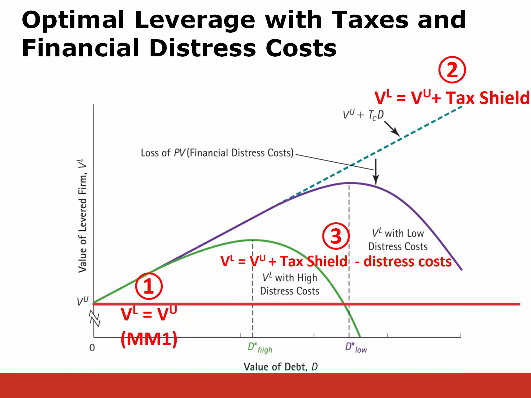
On this slide, distress costs are always equal to the difference between the dotted line and the curved colored line.

Steps 1-4: